[Deep Learning] Vanishing and Exploding Gradients | Weight Initialization | Batch Normalization | Layer Normalization

Vanishing Gradients

- usually occurs due to the fact that some activation functions squash the input into small values result in small gradients that result in negligible updates to the weights of the model

 

- Or sometimes the input values are small to begin with

 

: When backpropagation the gradient through long chains of computations, the gradient gets smaller and smaller

 

- causes the gradient of the parameters in the early layers to be very small.

- causes if the parameter space to have flat areas 

 

=> The parameters do not change too much during training and they will stay “almost” randomly initialized.

 

=> Solution :  Non-saturating activation functions

: avoid using Saturating Activation functions as activations of the hidden layers.

 

Saturating Activation Functions  : Sigmoid, Tanh

( two saturation points where the gradient is close to zero ) 

-> This causes the final gradient to be small as well. 

 

=> USE ReLU function (but could have vanishing gradient problem) 

 

=> Then, Use Leaky ReLU ( propagate a gradient > 0 even when x < 0) 

 

 

=>  Solution :  Gradient shortcuts

: add gradient shortcuts in the model.

 

Shorter Path ->  Fewer multiplications  -> Larger Gradient

 

(ex) Residual Networks, Skip Connections, DenseNet

 

 

=> + Solutions : Initialization, Normalization,

 

 

Exploding Gradients

: When backpropagation the gradient through long chains of computations, the gradient gets bigger and bigger.

 

- causes if the parameter space to have very steep areas 

- causes the gradient of the parameters in the early layers to be very big.

- occurs when the gradients become very large, leading to unstable learning

 

=> Solution :  Gradient Clipping.

One way to do gradient clipping involves forcing the gradient values (element-wise) to a specific maximum absolute value C.

- Limit the magnitude of gradients when they become too large

- Address the problem of exploding gradients by scaling down gradients that exceed a specified threshold.

 

 

 

 

Weight Initialization

: overcome various training challenges, improve the network's learning capabilities, and enable faster and more effective training.

 

1) Initialization based on Constant (Zero, Random) 

Zero Initialization -> NOT GOOD! 

 

Instead, Initialize parameters with Random Values

: having all parameters with the same value would render the network equivalent to having just one node in each layer to maintain the diversity and effectiveness of a neural network,

 

=> BUT, Randomly initializing the initial values only to fit specific conditions can lead to values becoming excessively large or small. This can cause the outputs of the layers to be erratic, making the learning process difficult

=> also vanishing gradient problem 

 

2) Probability distribution-based Initialization

causes the activation distributions to become non-uniform across the entire neural network as the depth of the layers increases.

 

=> BUT, it leads to non-homogeneous distributions of activations.

=> Consequently, this phenomenon contributes to the vanishing gradient problem as activation values tend to converge towards zero.

 

 

3) Variance Scaling Initialization - Xavier Initialization

: Variance Scaling Initialization, or Variance Scaling Technique, is a method that initializes weights based on values extracted from a probability distribution.

It dynamically adjusts the variance of this probability distribution for each weight.

 

https://www.geeksforgeeks.org/xavier-initialization/

Xavier initialization - GeeksforGeeks

 

 

 

Batch Normalization 

Normalization 

: input features take values on very different scalesor with very different biases.

-> applied the normalization to the input features

 

- popular normalization : Standardization

( scale each feature so that its mean is zeroand its variance is one )

 

 

Why Do we Need Batch Normalization? 

-> Internal Covariate Shift

: the phenomenon where, as neural networks become deeper, the input distribution of each layer undergoes changes.

 

-> During weight updates, since each layer learns based on the output of the previous layer, changes in the input distribution accumulate as they propagate through the layers, making the problem worsen. 

 

-> Even if the distribution of the previous layer changes, we can expect it to have a certain mean and variance. 

 

 

Batch Normalization

: It stabilizes the input distribution of each layer, ensuring that each layer can learn more effectively and in a stable manner.

 

- adjusting the mean and variance of the inputs for each batch of data, which helps prevent the input distributions from drifting significantly during training.

- the stability leads to faster convergence during training and allows for better overall performance of the neural network

 

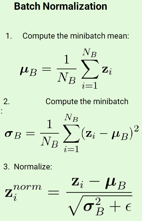
- Similar to input normalization, but computed at a minibatch level in the internal layers

 

- Add additional learnable parameters that allow the neural network to set a mean different than 0 and a variance different than 1.

gamma : scale, beta : shift

* The scale(gamma) and shift factors(beta) are learned from data though backpropagation

 

Why do we need extra parameter scale, shift factors?

- When batch normalization is applied, the weights are normalized to have a mean of 0 and a variance of 1. However, when ReLU is used as the activation function, negative values become 0.

 

=> To address this issue, the gamma and beta parameters are introduced. even after applying ReLU, the original negative values are not entirely reduced to 0, preventing the loss of information and ensuring that the benefits of normalization are not completely nullified.

 

 

How Batch Normalization Behave Different during the Training Time and Test(Inference) Time ? 

During Training:

1) Calculate the mean and variance of the input data within each mini-batch.
2) Normalizes the input data using the batch's mean and variance, scaling and shifting the data.

3) Keep track of two additional parameters, gamma (scale) and beta (shift), which are learned during training to make the normalization more effective.

 

During Testing (Inference):
1) Use the accumulated statistics from the training phase, which include the overall mean and variance of the entire dataset. 

( Since there are no mini-batch data available, the mean and variance calculated during the training process are used to normalize the inputs.)

2) Instead of calculating batch-wise statistics, it directly applies the previously learned gamma and beta to normalize the input data.

3) Ensure that the model behaves consistently and can make predictions on individual examples without needing a batch of data.

 

 

Effect of Batchnormalization 

The goal of Batch Normalization is to reduce the variation in values before applying activation.

-> If the changes in the hidden layer are not too extreme, it helps stabilize the training process.

 

 

- Regularization effect(avoid overfitting) 

=> Intuition: noise introduced from running mean and variance

=> as the mean and variance continuously change and also affect weight updates, it prevents the training from being dominated by a single weight direction 

=> less sensitive to weight Initialization in training

 

 

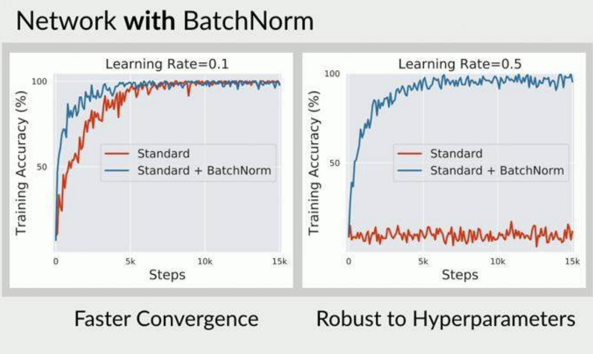
- It significantly speeds up training and generally leads to better convergence ( faster convergence ) 

- make the parameter space more “friendly” and easier to optimize.

- Can reach better testing accuracy

- possible to use larger learning rates, since batchnorm makes the network more stable during training

 

 

Disadvantage of Batchnormalization 

- It is influenced by the batch size.

=> If the batch size becomes too small, it may not exhibit a Gaussian distribution.

=> If the batch size becomes too large, parallelization efficiency in operations can decrease, and it may take longer to compute and incorporate gradients during training.

 

 

 

Layer Normalization 

: normalize over the neuron axis rather than the minibatch . 

 

- independently adjusts the values in each layer during training.

- stabilizes the distribution of values between layers, allowing the model to learn quickly and steadily.

- requires less hyperparameter tuning and helps keep the model simple.

- It does not depend on batch size. 

- The calculation methods during both training and testing are the same.

 

 

 

 

How Layer Normalization Behave During the Training Time and Test(Inference) Time ? 

During Training:
1) Calculate the mean and variance of the input features for each training example independently.
2) Normalize the input features for each example using its own mean and variance.
3) The normalization process is applied to the training data to help the model learn better representations.

 

During Testing (Inference):
1) Calculates the mean and variance for each input feature, but it uses the aggregated statistics from the training phase.
2) The same normalization process, utilizing the overall mean and variance, is applied to the test data.
3) This consistency between training and testing ensures that the model behaves similarly and makes predictions based on the learned statistics.