
Code&Data Insights
[Deep Learning] Optimization - Gradient Descent | Stochastic Gradient Descent | Mini-batch SGD 본문
[Deep Learning] Optimization - Gradient Descent | Stochastic Gradient Descent | Mini-batch SGD
paka_corn 2023. 11. 1. 11:08Optimization

- Training a machine learning model often requires solving Optimization problem
=> have to find the parameters of the function f that minimizes the loss function using the training data.
Problem in Optimization in Multi dimensional Spaces

- TOO MANY CRITICAL POINT! (critical points where f'(x) = 0)
=> local minima, maxima, and saddle points
How to Solve Optimization Problem?
Solution 1 : Find the Analytical Solution
1) compute the gradient f'(x)
2) find a closed-form expression where all the critical points
( hard to find the closed-form expression except for linear(simple) function)
3) test all critical points we found and choose ONE MINIMIZE THE LOSS!
Solution 2 : Find the Numerical Solution
: finding an approximate solution to the problem
1) Start from a set of candidate solutions(LOCAL OPTIMA)
2) Progressively improve the candidate solutions until convergence.
(The algorithm is sensitiveto the initialization point)
WHY LOCAL OPTIMA?
* find a global optimum - computationally demanding
* Some of them can find local optima only
(hill-climbing, coordinate descent, gradient descent)
* Local optimization is much faster than global optimization.
Gradient Descent
Gradient (Derivative)
: When we have more than one parameter we have to compute the partial derivatives over all the parameters
-> It is a vector that points in the direction of the greatest increase of the objective(loss)
Learning Rate
: a crucial factor, influences how quickly or slowly converges to an optimal solution.
* Changing the learning rate over the epochs can improve performance and reduce training time.
- The learning rate is a hyperparameter that determines how much the weights are adjusted with respect to the loss gradient.
- If lr is too small, it requires many updates and progresses very slow!
- If lr is too large, it causes drastic updates(divergent behavior)
=> too large - oscillation(진동)
=> much too large - instability(불안정)
Learning Rate Annealing
: reduce the learning rate while we train.
- new-bob annealing : reduce the learning rate when some conditions are met


Gradient Descent
- we update the parameter based on the gradient.
- proper initialization is IMPORTANT!
- each iteration uses the entire dataset to update the weights
Update Rules

wt+1 = wt − α∇wℒ(X,Y,wt)
Advantages and Disavantages
Disadvantages
- GD can get stuck in local optima
- difficult to apply to non-differentiable loss function
- require tuning the learning rate (+ batch size for SGD)
- can be costly (time & memory) since we need to evaluate the whole training dataset before we take one step towards the minimum.
(significantly more computation resources)
Batch Size
: number of samples in the minibatch
=> increase computational cost, but also accuracy

- Minibatch
: set of training samples used for computing the gradient.
Stochastic Gradient Descent (SGD)
: use noisy versions of the gradient, update the model's parameters using the gradient of the loss function with respect to a single training example(traditinally 1 batch) at a time.
- a single point(or a batch of points) are used in each iteration to update weights.
- It introduces some randomness in the learning process that helps the algorithm to escape from saddle points and local minima => Regularization Effect!
Update Rules

wt+1 = wt − α∇wl(x, y,wt)
Advantages and Disavantages
Advantages
- It converges faster compared to GD
- It can be shown to reach the global minimum in convex settings
- SGD much more scalable in large datasets compared to GD
- Local minumum in non-convex functions obtained by SGD are “close” to global minimum.
=> SGD naturally introduces some regularization that yields better generalization properties.
Disadvantages
- Inefficient computation and lead to noisy updates
- Due to the randomness, convergence can be unstable, and noise can be present.
- the error function is not as well minimized as in the case of GD
Mini-batch SGD
: updating the model's parameters using a small random subset (mini-batch) of the training data at each iteration.
Update Rules
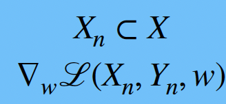
wt+1 = wt − α∇wℒ(Xn,Yn,wt)
Advantages and Disavantages
Advantages
- can be seen as obtaining a lower variance gradient estimate but without need for full batch
(compromise between GD and SGD)
- Forward and Backward processing is often more efficient on single GPU
* SGD with small mini-batch can find flatter minimum and that flat minimum generalize better
"Flat regions"
- Refer to areas in the loss function where the gradient is close to zero.
- In such regions, the gradient doesn't change abruptly, allowing gradient descent to converge quickly.
- In flat regions, gradient descent optimizes rapidly, leading to stable convergence when updating the model's weights.
Disadvantages
- Initialization Sensitivity
- Plateaus(regions of very small gradient) and Saddle Points(points where the gradient is zero but not necessarily a minimum).


